SURVIVAL ANALYSIS
Survival analysis is a branch of statistics that studies the time to event. Please feel free to read my two part series on the introduction to survival analysis from my Medium stories. https://medium.com/@Statistician_Leboo.
This is a survival analysis project using the lung cancer data found from the survival package in R.
Reading the data
The data is in the survival package. This package comes pre-installed in base R.
library(survival)
lung_data <- lung
1. EDA
Loading required packages
library(tidyverse)
library(dplyr)
library(mice)
library(Hmisc)
library(ggplot2)
Describing the data
The data has 10 variables of different types. Before performing description of the data using the describe command from the Hmisc package, factor variables are converted from numeric so as to not give misleading insights. The variable inst is dropped has it offers no significant insights.
lung_data %>%
  select(-inst) %>%
  mutate(status=as.factor(status),
         sex=as.factor(sex),
         ph.ecog=as.factor(ph.ecog),
         pat.karno=as.factor(pat.karno)) %>%
  describe()
## .
##
##  9  Variables      228  Observations
## --------------------------------------------------------------------------------
## time
##        n  missing distinct     Info     Mean      Gmd      .05      .10
##      228        0      186        1    305.2      228     53.0     80.4
##      .25      .50      .75      .90      .95
##    166.8    255.5    396.5    616.3    733.6
##
## lowest :    5   11   12   13   15, highest:  840  883  965 1010 1022
## --------------------------------------------------------------------------------
## status
##        n  missing distinct
##      228        0        2
##
## Value          1     2
## Frequency     63   165
## Proportion 0.276 0.724
## --------------------------------------------------------------------------------
## age
##        n  missing distinct     Info     Mean      Gmd      .05      .10
##      228        0       42    0.999    62.45    10.31    45.35    50.00
##      .25      .50      .75      .90      .95
##    56.00    63.00    69.00    74.00    75.00
##
## lowest : 39 40 41 42 43, highest: 76 77 80 81 82
## --------------------------------------------------------------------------------
## sex
##        n  missing distinct
##      228        0        2
##
## Value          1     2
## Frequency    138    90
## Proportion 0.605 0.395
## --------------------------------------------------------------------------------
## ph.ecog
##        n  missing distinct
##      227        1        4
##
## Value          0     1     2     3
## Frequency     63   113    50     1
## Proportion 0.278 0.498 0.220 0.004
## --------------------------------------------------------------------------------
## ph.karno
##        n  missing distinct     Info     Mean      Gmd
##      227        1        6    0.934    81.94    13.48
##
## lowest :  50  60  70  80  90, highest:  60  70  80  90 100
##
## Value         50    60    70    80    90   100
## Frequency      6    19    32    67    74    29
## Proportion 0.026 0.084 0.141 0.295 0.326 0.128
## --------------------------------------------------------------------------------
## pat.karno
##        n  missing distinct
##      225        3        8
##
## lowest : 30  40  50  60  70 , highest: 60  70  80  90  100
##
## Value         30    40    50    60    70    80    90   100
## Frequency      2     2     4    30    41    51    60    35
## Proportion 0.009 0.009 0.018 0.133 0.182 0.227 0.267 0.156
## --------------------------------------------------------------------------------
## meal.cal
##        n  missing distinct     Info     Mean      Gmd      .05      .10
##      181       47       60    0.996    928.8    421.9      338      413
##      .25      .50      .75      .90      .95
##      635      975     1150     1225     1425
##
## lowest :   96  131  169  238  271, highest: 1500 2200 2350 2450 2600
## --------------------------------------------------------------------------------
## wt.loss
##        n  missing distinct     Info     Mean      Gmd      .05      .10
##      214       14       53    0.995    9.832    13.92    -5.00    -1.70
##      .25      .50      .75      .90      .95
##     0.00     7.00    15.75    28.00    33.35
##
## lowest : -24 -16 -15 -13 -11, highest:  39  49  52  60  68
## --------------------------------------------------------------------------------
The summary command can also be used to generate further summary statistics.
lung_data %>%
  select(-inst) %>%
  mutate(status=as.factor(status),
         sex=as.factor(sex),
         ph.ecog=as.factor(ph.ecog),
         pat.karno=as.factor(pat.karno)) %>%
  summary()
##       time        status       age        sex     ph.ecog       ph.karno
##  Min.   :   5.0   1: 63   Min.   :39.00   1:138   0   : 63   Min.   : 50.00
##  1st Qu.: 166.8   2:165   1st Qu.:56.00   2: 90   1   :113   1st Qu.: 75.00
##  Median : 255.5           Median :63.00           2   : 50   Median : 80.00
##  Mean   : 305.2           Mean   :62.45           3   :  1   Mean   : 81.94
##  3rd Qu.: 396.5           3rd Qu.:69.00           NA's:  1   3rd Qu.: 90.00
##  Max.   :1022.0           Max.   :82.00                      Max.   :100.00
##                                                              NA's   :1
##    pat.karno     meal.cal         wt.loss
##  90     :60   Min.   :  96.0   Min.   :-24.000
##  80     :51   1st Qu.: 635.0   1st Qu.:  0.000
##  70     :41   Median : 975.0   Median :  7.000
##  100    :35   Mean   : 928.8   Mean   :  9.832
##  60     :30   3rd Qu.:1150.0   3rd Qu.: 15.750
##  (Other): 8   Max.   :2600.0   Max.   : 68.000
##  NA's   : 3   NA's   :47       NA's   :14
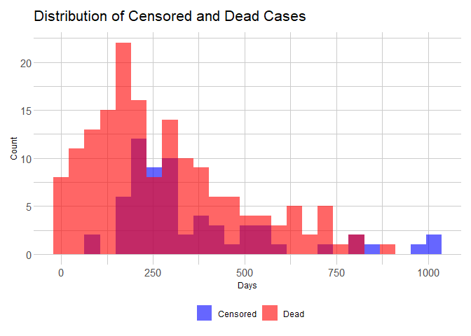
Visualizing the distribution of Censored and Dead Cases
From the data, the event of interest is death. As explained in the theoretical blog, censoring occurs when the event of interest was not recorded during the study.
ggplot(lung_data, aes(x = time, fill = factor(status))) +
  geom_histogram(bins = 25, alpha = 0.6, position = "identity") +
  scale_fill_manual(values = c("blue", "red"), labels = c("Censored", "Dead")) +
  ezfun::theme_ezbasic() +
  labs(x = "Days",
       y = "Count",
       title = "Distribution of Censored and Dead Cases")
Visualizing Continuous Variables
This set of code was obtained from Rpubs. First of all, select continuous variables, then convert them into long format. Plot a histogram of the data faceting all variables. The colour schemes in this plot are from the ezfun package developed by Emily Zabore.
trl=lung_data %>%
        select(status, age, meal.cal, pat.karno, ph.karno, time, wt.loss) %>%
        pivot_longer(-one_of("status")) %>%
        mutate(had_event=ifelse(status==1,"Censored", "Died"))
ggplot(trl) +
  aes(x = value, colour = had_event) +
  geom_density(adjust = 1L, fill = "#112446") +
  scale_color_brewer(palette = "Set1", direction = 1) +
  labs(title = "Distribution Across Continuous Variables",
    color = "Status") +
  hrbrthemes::theme_modern_rc() +
  theme(legend.position = "top",
    plot.title = element_text(face = "bold",hjust = 0.5),
    strip.text.x = element_text(size = 12, color = "cyan", face = "bold.italic"),
    strip.text.y = element_text(size = 12, color = "red", face = "bold.italic")) +
  facet_wrap(. ~ name, scales="free")
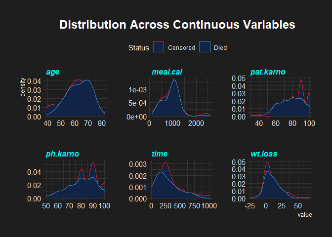 From the plot above, the distributions of the continuous variables do not display a normal distribution. However, I won’t dive much into checking for normality.
Generating Crosstabs for categorical variables; sex, event and ph.ecog
Patient’s performance status (ECOG), is a standardized criteria used to
measure how a disease impacts a patient’s daily living abilities. The
scale assigns a scale from 0-5 as displayed in the figure below. 
In the chunks below, we tabulate the three categorical variables. ph.ecog is the scale assigned by a physician to a patient depending on their living abilities.
library(gt)
library(janitor)
options(dplyr.summarise.inform=FALSE) #to prevent warnings from being displayed
lung_data %>%
  select(time,sex,status,ph.ecog) %>%
  drop_na() %>%

  mutate(sex=as.factor(ifelse(sex==1,"Male","Female")),
         status=as.factor(ifelse(status==1,"Censored", "Dead")),
         ph.ecog=as.factor(ifelse(ph.ecog==0,"0: Fully Active",
                                  ifelse(ph.ecog==1,"1: Restricted Physically",
                                                                    ifelse(ph.ecog==2,"2: In bed<50% a day",ifelse(ph.ecog==3,"3: In bed>50% a day",
                                                                           ifelse(ph.ecog==4,"4: Bed Bound", "5: Dead"))))))) %>%
  group_by(sex,ph.ecog,status) %>%
  summarise(Count=n()) %>%
  group_modify(~.x %>% adorn_totals(where = "row")) %>%
  gt()%>%
  gtsave(filename="catVars.html")
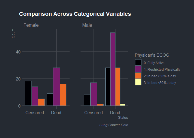
The data had 228 observations. 63 (27.63%) were censored and 165 (72.37%) were recorded to have experienced the event of death. 90 (39.47%) were female while 138 (61.53%) were male. 63 (27.6%) of patients had a physicians ECOG score of 0, 113 (49.6%) had a score of 1, 50 (21.9%) had 2 while 1 (0.4%) had a score of 1 and 1 record had missing entry. The figure below shows the distribution of patients across the three variables.
lung_data %>%
  select(time,sex,status,ph.ecog) %>%
  drop_na() %>%
  mutate(sex=as.factor(ifelse(sex==1,"Male","Female")),
         status=as.factor(ifelse(status==1,"Censored", "Dead")),
         ph.ecog=as.factor(ph.ecog),
         ph.ecog1=as.factor(ifelse(ph.ecog==0,"0: Fully Active",
                                  ifelse(ph.ecog==1,"1: Restricted Physically",
                                                                    ifelse(ph.ecog==2,"2: In bed<50% a day",ifelse(ph.ecog==3,"3: In bed>50% a day",
                                                                           ifelse(ph.ecog==4,"4: Bed Bound", "5: Dead"))))))) %>%
  ggplot() +
  aes(x = status, fill = ph.ecog1) +
  geom_bar(position = "dodge")+
  scale_fill_viridis_d(option = "inferno", direction = 1) +
  labs(x = "Status",y = "Count",
    title = "Comparison Across Categorical Variables",
    caption = "Lung Cancer Data",
    fill = "Physican's ECOG") +
  hrbrthemes::theme_ft_rc() +
  theme(plot.title = element_text(size = 14L,hjust = 0.5),
    plot.caption = element_text(face = "italic")) +
  facet_wrap(vars(sex))
Hypothesis Testing
Test for Independence Among Categorical Variables
Chi-square goodness of fit test was used to assess the independence of these variables. The test was done 0.05 level of significance.
Hypothesis Null: Independence among the variables. Alternative: Dependence among the variables.
Rejection Criteria If p-value is less than alpha, the null hypothesis is rejected.
To perform this, cross tables were build using the gmodels package that computes chi-square values.
library(gmodels)
cat_vars<-lung_data %>%
  select(time,sex,status,ph.ecog) %>%
  drop_na() %>%
  mutate(sex=as.factor(ifelse(sex==1,"Male","Female")),
         status=as.factor(ifelse(status==1,"Censored", "Dead")),
         ph.ecog=as.factor(ifelse(ph.ecog==0,"0: Fully Active",
                                  ifelse(ph.ecog==1,"1: Restricted Physically",
                                                                    ifelse(ph.ecog==2,"2: In bed<50% a day",ifelse(ph.ecog==3,"3: In bed>50% a day",
                                                                           ifelse(ph.ecog==4,"4: Bed Bound", "5: Dead"))))))) %>%
  group_by(sex,ph.ecog,status)

CrossTable(cat_vars$sex, cat_vars$status,prop.r = F, prop.t = T,
           prop.chisq = F,prop.c = F, chisq=T)
##
##
##    Cell Contents
## |-------------------------|
## |                       N |
## |         N / Table Total |
## |-------------------------|
##
##
## Total Observations in Table:  227
##
##
##              | cat_vars$status
## cat_vars$sex |  Censored |      Dead | Row Total |
## -------------|-----------|-----------|-----------|
##       Female |        37 |        53 |        90 |
##              |     0.163 |     0.233 |           |
## -------------|-----------|-----------|-----------|
##         Male |        26 |       111 |       137 |
##              |     0.115 |     0.489 |           |
## -------------|-----------|-----------|-----------|
## Column Total |        63 |       164 |       227 |
## -------------|-----------|-----------|-----------|
##
##
## Statistics for All Table Factors
##
##
## Pearson's Chi-squared test
## ------------------------------------------------------------
## Chi^2 =  13.27044     d.f. =  1     p =  0.0002696233
##
## Pearson's Chi-squared test with Yates' continuity correction
## ------------------------------------------------------------
## Chi^2 =  12.18955     d.f. =  1     p =  0.0004805786
##
##
16.3% of the observations were female and were censored, while 23.3% were female and experienced death. On the other hand, 11.5% were male and were censored while 48.9% were male and experienced death. The Chi-square test was used to check for independence between sex and event. The null hypothesis in this case was existence of dependence between the two tested at 5% alpha level. The test reported a p<0.001 hence the null hypothesis was rejected. The test concluded that there existed sufficient statistical evidence at 5% significance to disapprove the claim that event was dependent on sex of patients.
CrossTable(cat_vars$ph.ecog, cat_vars$status,prop.r = F, prop.c = F,
           prop.t = T, prop.chisq = F, chisq=T)
  ##    Cell Contents
## |-------------------------|
## |                       N |
## |         N / Table Total |
## |-------------------------|
##
##
## Total Observations in Table:  227
##
##
##                          | cat_vars$status
##         cat_vars$ph.ecog |  Censored |      Dead | Row Total |
## -------------------------|-----------|-----------|-----------|
##          0: Fully Active |        26 |        37 |        63 |
##                          |     0.115 |     0.163 |           |
## -------------------------|-----------|-----------|-----------|
## 1: Restricted Physically |        31 |        82 |       113 |
##                          |     0.137 |     0.361 |           |
## -------------------------|-----------|-----------|-----------|
##      2: In bed<50% a day |         6 |        44 |        50 |
##                          |     0.026 |     0.194 |           |
## -------------------------|-----------|-----------|-----------|
##      3: In bed>50% a day |         0 |         1 |         1 |
##                          |     0.000 |     0.004 |           |
## -------------------------|-----------|-----------|-----------|
##             Column Total |        63 |       164 |       227 |
## -------------------------|-----------|-----------|-----------|
##
##
## Statistics for All Table Factors
##
##
## Pearson's Chi-squared test
## ------------------------------------------------------------
## Chi^2 =  12.31869     d.f. =  3     p =  0.006367498
##
##
##
Of the 63 patients who had ph.ecog scores of 0: Fully Active, 11.5% of the observations were censored while 16.3% experienced death. 113 patients who had ph.ecog scores of 1: Restricted Physically, 13.7% were censored while 36.1% experienced death. 50 patients had ph.ecog scores of 2: In bed less than 50% a day. 2.6% were censored and 19.4% experienced death. Only 1 patient,(0.4%) had a ph.ecog score of 3: In bed more than 50% a day and the patient experienced death. A Chi-square test of independence between ph.ecog score and event reported a p<0.01 implying that there wast sufficient evidence at 5% alpha level to suffice the dependence of experiencing event and ph.ecog.
Do both women and men experience death at the same rates?
A two-sample z-test was used to assess the difference between the males and females who died of lung cancer. The test was done 0.05 level of significance. Dummy variables were generated and z-test was used since the data has more than 30 variables. An assumption was made that the data is normal hence the parametric approach.
Hypothesis Null: No difference between males and females. Alternative: There is a difference between males and females.
Rejection Criteria If p-value is less than alpha, the null hypothesis is rejected.
library(BSDA)
dead<-lung_data %>%
  select(status,sex) %>%
  subset(status==2) %>%
  mutate(isMale=as.numeric(ifelse(sex==1,"1","0")),
         isFemale=as.numeric(ifelse(sex==2,"1","0")))


z.test(x=dead$isMale,y=dead$isFemale, mu=0, sigma.x=(sd(dead$isMale)),sigma.y=(sd(dead$isMale))
       ,alternative = 'two.sided', conf.level=0.95)
##
##  Two-sample z-Test
##
## data:  dead$isMale and dead$isFemale
## z = 6.9344, p-value = 4.078e-12
## alternative hypothesis: true difference in means is not equal to 0
## 95 percent confidence interval:
##  0.2565100 0.4586415
## sample estimates:
## mean of x mean of y
## 0.6787879 0.3212121
There was significant effect for sex for individual who experienced death, Z(328) = 6.9334, p<.001. Males (M=0.6788, SD = 0.4684) experienced death more than females (M = 0.3212, SD = 0.4684). The null hypothesis is therefore rejected. The test concludes, there exists sufficient statistical evidence at 0.05 level of significance to deny the claim that the proportion of males and females that died of lung cancer was equal.
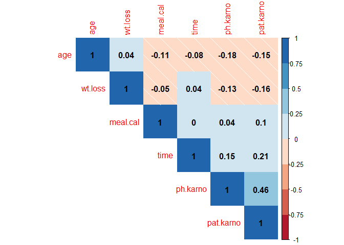
Correlation Analysis Among Numeric Variables
library(corrplot)
library(RColorBrewer)
num_data <- lung_data %>%
                  select(age, ph.karno, pat.karno, meal.cal, wt.loss, time) %>%
                  replace(is.na(.), 0)

corrs = cor(num_data)
corrplot(corrs, type="upper", order="hclust", method="shade",
         col=brewer.pal(n=8, name="RdBu"), addCoef.col = "black")
2. Survival Models
2.1 Kaplan Meier Model
This is one of the most used models in Survival Analysis. The project builds some KM models as shown below.
Model 1
In this model, we look into the time to event and status of event of interest.
attach(lung_data)
model1_kaplan<-survfit(Surv(time,status)~1,
                       type="kaplan-meier")
model1_kaplan
detach()
## Call: survfit(formula = Surv(time, status) ~ 1, type = "kaplan-meier")
##
##        n events median 0.95LCL 0.95UCL
## [1,] 228    165    310     285     363
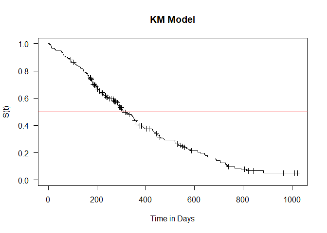
There were 228 observations with the median time to event being recorded at 165 (285,363) days. Use the summary() command to view the survival at different times and the confidence intervals. Please note that if the data set is small, the confidence intervals will be wide.
summary(model1_kaplan)
Visualizing Model 1
Below are some visualizations for the first model.
plot(model1_kaplan, conf.int = F, xlab = "Time in Days",
     ylab = "S(t)", main="KM Model", las=1, mark.time = T)
# Median survival
abline(h=0.5, col="red")
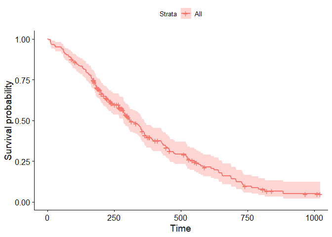
 You can visualize the model using the ggsurvplot function.
library(survminer)
attach(lung_data)
mdl<-survfit(Surv(time,status)~1)
ggsurvplot(fit=mdl, data=lung_data)
detach()
Model 2
In this model, we incorporate the variable sex into the model.
lung_data<-lung_data %>% mutate(sex=ifelse(sex==1,"Male","Female"))
attach(lung_data)
model2_kaplan<-survfit(Surv(time,status)~sex)
model2_kaplan
## Call: survfit(formula = Surv(time, status) ~ sex)
##              n events median 0.95LCL 0.95UCL
## sex=Female  90     53    426     348     550
## sex=Male   138    112    270     212     310
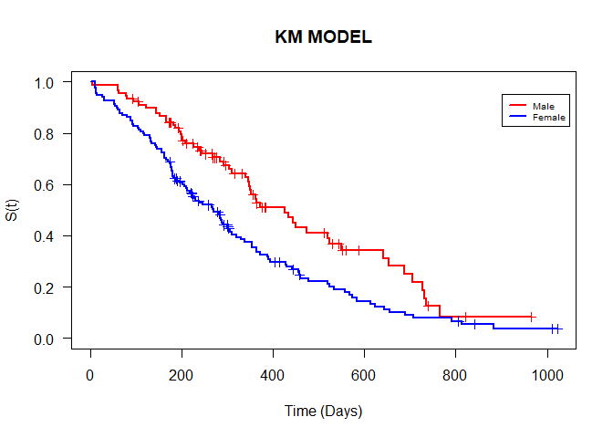
The summary of the model shows that there were a total of n=228 observations. 53 out of the 90 females experienced death and their median time to event was 426 (348,550) days. 112 out of the 138 males experienced death with their median time to event was 270 (212,310) days. You can also generate a summary fpr the model.
summary(model2_kaplan)
Visualizing Model 2
plot(model2_kaplan, conf.int = F, xlab = "Time (Days)", ylab = "S(t)",
     main="KM MODEL", col = c("red", "blue"), las=1, lwd=2, mark.time = T)
legend(900,0.95, legend = c("Male", "Female"), lty = 1, lwd=2, col = c("red", "blue"),
       bty = "", cex=0.6)
 The ggsurvplot function allows for the comparison of the survival models and also the addition of the risk table. By default the test used is the log-rank test.
library(ggsci)
ggsurvplot(fit=model2_kaplan, data=lung_data, conf.int = TRUE, palette ="aaas" ,
           size =1, linetype = "strata" ,pval = TRUE, risk.table = TRUE, method="log-rank",
           tables.col="strata", tables.text=FALSE)
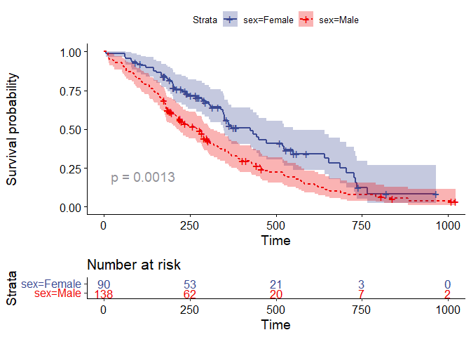
The null hypothesis in a log-rank test is that there is no difference between the curves. From the plot above, a p-value of 0.0013 was returned. Using an alpha level of 0.05, the null hypothesis is rejected. There exist sufficient statistical evidence at 5% alpha level to suffice a difference between the survival curves of males and females in the lung dataset.
You can compare survival rates to other variables in the data. However, you can’t add many X variables since you will have many survival curves. The KM model only allows for categorical explanatory model.
attach(lung_data)
model3_kaplan<-survfit(Surv(time,status)~ph.ecog+sex,
                       type="kaplan-meier")
model3_kaplan
detach()
## Call: survfit(formula = Surv(time, status) ~ ph.ecog + sex, type = "kaplan-meier")
##
##    1 observation deleted due to missingness
##                        n events median 0.95LCL 0.95UCL
## ph.ecog=0, sex=Female 27      9    705     350      NA
## ph.ecog=0, sex=Male   36     28    353     303     558
## ph.ecog=1, sex=Female 42     28    450     345     687
## ph.ecog=1, sex=Male   71     54    239     207     363
## ph.ecog=2, sex=Female 21     16    239     199     444
## ph.ecog=2, sex=Male   29     28    166     105     288
## ph.ecog=3, sex=Male    1      1    118      NA      NA
2.2 Cox Proportional Hazards Model
This model obtains the hazard ratio in form of beta coefficients. However, we do not obtain the baseline hazard. Cox models allows for the inclusion of numerous X variables both numeric and categorical.
Model 1
The first model has the variable sex has the co-variate. If you use the original data to build the model, note that the variable sex has not been coded as a factor. Hence be keen on the reference point of the interpretation.
attach(lung_data)
model1_cox<-coxph(Surv(time,status)~sex)
summary(model1_cox)
detach()
## Call:
## coxph(formula = Surv(time, status) ~ sex)
##
##   n= 228, number of events= 165
##
##           coef exp(coef) se(coef)     z Pr(>|z|)
## sexMale 0.5310    1.7007   0.1672 3.176  0.00149 **
## ---
## Signif. codes:  0 '***' 0.001 '**' 0.01 '*' 0.05 '.' 0.1 ' ' 1
##
##         exp(coef) exp(-coef) lower .95 upper .95
## sexMale     1.701      0.588     1.226      2.36
##
## Concordance= 0.579  (se = 0.021 )
## Likelihood ratio test= 10.63  on 1 df,   p=0.001
## Wald test            = 10.09  on 1 df,   p=0.001
## Score (logrank) test = 10.33  on 1 df,   p=0.001
From the results, we have 165 individuals experiencing death out of a total of 228. The coefficients table displays that sex was a significant co-variate; p(0.00149). From the output, at any given point of time, the log instantaneous risk of death is0.531 higher for males as compared to females. This means that the risk of death in males is higher than than of females. The hazard ratio is 1.7007. This tells us that, at any given point in time, Males are 1.7 times at risk of death as compared to Females ignoring all other variables. The hazard of death in Males at any given point of time lies between (1.23,2.36) times that of Females. Based on the evidence above, we can conclude that the Males are at more risk of death as compared to Females. This is because; a. The p-value is less than 0.05 b. The confidence interval does not contain 1. The tests below the output can confirm this.
It can be estimated that at any given point of time, Males are 70% more likely to die as compared to females holding all other factors constant.
The Cox model does not compute the survival since we have no baseline hazard. You can try to build another model with more covariates as shown below. However, I will not explain the results.
Model 2
attach(lung_data)
model2_cox<-coxph(Surv(time,status)~ph.karno+sex+meal.cal+wt.loss+ph.ecog)
summary(model2_cox)
detach()
## Call:
## coxph(formula = Surv(time, status) ~ ph.karno + sex + meal.cal +
##     wt.loss + ph.ecog)
##
##   n= 170, number of events= 123
##    (58 observations deleted due to missingness)
##
##                coef  exp(coef)   se(coef)      z Pr(>|z|)
## ph.karno  0.0172016  1.0173504  0.0107977  1.593 0.111142
## sexMale   0.5709145  1.7698849  0.1976375  2.889 0.003868 **
## meal.cal -0.0001044  0.9998956  0.0002547 -0.410 0.681983
## wt.loss  -0.0118639  0.9882062  0.0075110 -1.580 0.114213
## ph.ecog   0.8020020  2.2300010  0.2157204  3.718 0.000201 ***
## ---
## Signif. codes:  0 '***' 0.001 '**' 0.01 '*' 0.05 '.' 0.1 ' ' 1
##
##          exp(coef) exp(-coef) lower .95 upper .95
## ph.karno    1.0174     0.9829    0.9960     1.039
## sexMale     1.7699     0.5650    1.2015     2.607
## meal.cal    0.9999     1.0001    0.9994     1.000
## wt.loss     0.9882     1.0119    0.9738     1.003
## ph.ecog     2.2300     0.4484    1.4611     3.404
##
## Concordance= 0.638  (se = 0.031 )
## Likelihood ratio test= 24.4  on 5 df,   p=2e-04
## Wald test            = 23.73  on 5 df,   p=2e-04
## Score (logrank) test = 24.22  on 5 df,   p=2e-04
Thanks for going through this content. Survival analysis is such a wide field. I hope this simple project gives insights on the concepts of survival analysis. See you on the next one.
References
Read more about these models from the references below. Cox Proportional-Hazards Model. Statistical Tools for High-Throughput Data Analysis (STHDA) Prof. Mike Marin. Survival Analysis| Concepts and Implemntation in R.