Introduction
Design of Experimen refers to the process of planning the experiment so that the appropriate data will be collected which may be analyzed by a statistical method. Design and analysis of experiments is a branch of statistics that is crucial and is applied in various sectors and industries such as health, agrigiculture and engineering.
There are may designs of experiments; Completely Randomized Design (CRD) Randomized Bleck Design (RBD) Latin Sqaure Designs (LSD) Factorial Experiments
In this blog, we will discuss performing CRD in R
Completely Randomized Design
This design contains one factor and thus only one way classification the general staistical model is: Yij=µ+αi+εij,
Where:
µ is the overall(grand) mean common to all treatment. It is the mean yield in the absence of the treatment effect of the experiment.
σ²εij is the random error of the jth observation receiving the ith treatment and is assumed to be N~iid(0, σ²)
εij is the random error of the jth observation receiving the ith treatment and is assumed to be N~iid(0, σ²)
The hypothesis under test is:
Null- αi=0, for all i
Alternative- αi≠0, for any i
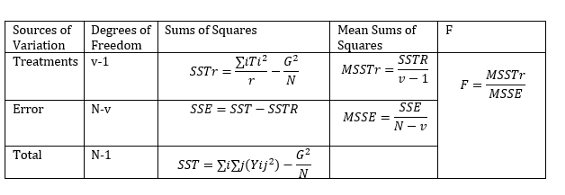
To perform manual ANOVA we follow the table below

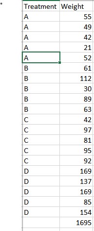
Find the dataset below; https://github.com/StatisticianLeboo/statistics-topics/tree/ANOVA

CRD
Example 1
The data contains 4 tropical food stuffs A, B, C, and D tried on 20 chicks. Analyze the data at 5% level of significance.
Solution
 We compare the computed F value with the tabulated one from the F tables 5% (3,16)=3.24. Since the tabulated value is small you reject the null hypothesis and conclude that the treatments vary significantly and do not have similar effect on the chicks.
An additional test; LSD is used to find which of the foods is mostly significant.
In R, we perform the analysis as follows:
library(readxl)
chicks <- read_excel("chics.xlsx")
 Set the treatment column into factors
chicks$Treatment<-as.factor(chicks$Treatment)
Performing ANOVA
Method 1
mod1<-aov(Weight~Treatment, data = chicks)
summary(mod1)
##             Df Sum Sq Mean Sq F value   Pr(>F)
## Treatment    3  26235    8745   12.11 0.000218 ***
## Residuals   16  11559     722
## ---
## Signif. codes:  0 '***' 0.001 '**' 0.01 '*' 0.05 '.' 0.1 ' ' 1
## 5 observations deleted due to missingness
Method 2
chicksmodel<-lm(Weight~Treatment, data = chicks)
anova(chicksmodel)
## Analysis of Variance Table
##
## Response: Weight
##           Df Sum Sq Mean Sq F value   Pr(>F)
## Treatment  3  26235  8745.0  12.105 0.000218 ***
## Residuals 16  11559   722.4
## ---
## Signif. codes:  0 '***' 0.001 '**' 0.01 '*' 0.05 '.' 0.1 ' ' 1
LSD Test
library(agricolae)
LSD.test(chicksmodel,"Treatment", console = TRUE)
##
## Study: chicksmodel ~ "Treatment"
##
## LSD t Test for Weight
##
## Mean Square Error:  722.425
##
## Treatment,  means and individual ( 95 %) CI
##
##   Weight      std r       LCL       UCL Min Max
## A   43.8 13.62718 5  18.31833  69.28167  21  55
## B   71.0 31.02418 5  45.51833  96.48167  30 112
## C   81.4 22.87575 5  55.91833 106.88167  42  97
## D  142.8 34.90272 5 117.31833 168.28167  85 169
##
## Alpha: 0.05 ; DF Error: 16
## Critical Value of t: 2.119905
##
## least Significant Difference: 36.03652
##
## Treatments with the same letter are not significantly different.
##
##   Weight groups
## D  142.8      a
## C   81.4      b
## B   71.0     bc
## A   43.8      c
From the LSD, it is clear that treatment D is the most effective. There is no much difference between C and B, whereas A has the least treatment effect.
Example 2
The data contains the amount of electricity used in KWh in three towns. Test at 5% significance whether the amount of electricity used is the same in the 3 towns. The steps are as example 1
library(readxl)
electricity <- read_excel("electricity.xlsx")

#Set the treatment variable to factor
electricity$Town<-as.factor(electricity$Town)
model2<-aov(Electricity_Used~Town, data=electricity)
summary(model2)
##             Df Sum Sq Mean Sq F value Pr(>F)
## Town         2  150.6   75.30   2.705  0.085 .
## Residuals   27  751.6   27.84
## ---
## Signif. codes:  0 '***' 0.001 '**' 0.01 '*' 0.05 '.' 0.1 ' ' 1