This was a research project undertaken by my classmates in which I was proud to be associated with. The are;
- EMMACULATE WANYAGA NYAGA
- MARIANE ACHIENG MAKOKHA
- OKARI MARYFINE SIGHALA
- MARLINE WESONGA
- NYALITA OLIVIA
This article otlines some of the analysis undertaken during the project. It however does not conclude the findings obatined in the research.
ABSTRACT
Performance Monitoring for Action project (PMA) is a project that collects various metrics concerning reproductive health. The data for this study was from a survey carried out in 2018 in Kenya across 11 counties and contained 25127 individuals whose various metrics were collected.
Objectives
To determine the preferred method of family planning among women of the reproductive age (15-49) in Kenya, with a choice of preference. The objective was accomplished through the analyses described in this article. Feel free to share your views and complements.
Loading the Data and Required Packages
library(readr)
library(knitr)
library(dplyr)
library(ggplot2)
library(reshape2)
library(tidyr)
library(stringr)
library(broom)
PMA_DATA <- read_csv("PMA2018_KER7_HHQFQ_2Dec2019.csv")
Some basic descriptives.
Distribution of women within the study criteria in percentage form
kable(PMA_DATA%>%
  select(county,age,gender, current_method) %>%
  subset(gender==2) %>%
  filter(between (age,15,49)) %>%
  group_by(county) %>%
  summarise(total=n()) %>%
  mutate(rate=round(((total/sum(total))*100),2),
         ratio=paste0(rate, "%")) %>%
    select(-3))
| county | total | ratio |
|---|---|---|
| 1 | 581 | 10.06% |
| 2 | 542 | 9.38% |
| 3 | 484 | 8.38% |
| 4 | 587 | 10.16% |
| 5 | 553 | 9.57% |
| 6 | 589 | 10.2% |
| 7 | 547 | 9.47% |
| 8 | 490 | 8.48% |
| 9 | 412 | 7.13% |
| 10 | 517 | 8.95% |
| 11 | 474 | 8.21% |
Most preferred family planning method
The study focuses on women aged(15-49) -99 values are recoded as No response
FP_preferred<-PMA_DATA %>%
  select(age,gender, current_method) %>%
  mutate(age=as.numeric(age)) %>%
  subset(gender==2) %>%
  filter(between (age,15,49)) %>%
  group_by(current_method) %>%
  summarize(total=n()) %>%
  drop_na()
FP_preferred$current_method[FP_preferred$current_method== "-99"]<-"No Response"
Further Summary Statistics were derived using Ms. Excel as it was much easier to analyze individuals who used one or more than one family planning procedure. 2498 (43%) of women of reproductive age were currently using at least one family planning method. 2 women out of the 5776 offered no response on their use of family planning methods. Of the women who were currently using family planning methods, 2368 (94.7%) reported to use one family planning method while 5.3% ,130 women reported to use more than one family planning method simultaneously. Of the women who currently use a single-family planning method, 39.74% (941) were reported to use injectables this being the most preferred method in this cohort whereas diaphragm method was the least preferred with 0.13% (3) women being reported to be currently using this method.
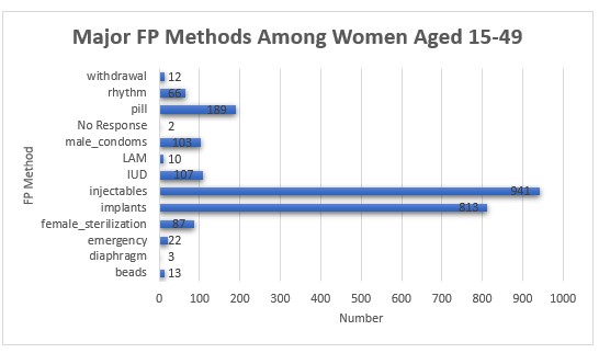
Of the women who use more than one FP method, pills and injectables were reported to be the most preferred combination with 20 women (15.38) of them choosing this combination.
Awareness to FP
To find the individuals who were aware of at least a single FP method, logical operations of OR is used. It is applied on the heard of columns and a nested if command is used to generate a column indicating awareness rates.
FP_access<-PMA_DATA %>%
  select(age,gender, current_method,heard_female_sterilization:heard_other) %>%
  mutate(age=as.numeric(age)) %>%
  subset(gender==2) %>%
  filter(between (age,15,49)) %>%
  select(heard_female_sterilization:heard_other) %>%
  drop_na()

fpheard<-colnames(FP_access)
fpheard_values<-tibble(colSums(FP_access))
accessfp<-data.frame(fpheard)
d<-data.frame(accessfp,fpheard_values)
FP_access2<-d %>%
  mutate(Number_of_individuals=colSums(FP_access),
         Rate=round((Number_of_individuals/sum(Number_of_individuals))*100,2),
         Awareness_Rate=paste0(Rate, "%"),
         Not_Aware=nrow(FP_access)-Number_of_individuals) %>%
  select(-colSums.FP_access.)
In this objective, the study was keen to investigate what is the awareness rate of major FP methods among the subjects. The major family planning methods are as follows;
• Female sterilization • Male sterilization • Implants • IUD • Injectables • Pills • Emergency • Male condoms • Female condoms • Diaphragm • Foam jelly • Beads • LAM • Rhythm • Withdrawal
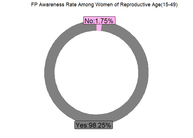
5622 out of 5722 women of reproductive age were aware of at least one major reproductive method this translate to an overall awareness rate of 98.25% as shown in figure 2 below. Note that this part of the analysis excluded women who chose not to respond.
Male condoms had the highest awareness rate of 10.85% with 5370 women of reproductive age being reported to have heard of this FP method. Foam jelly had the lowest awareness rate with only 645 (1.30%) of women being reported to have heard about this FP method. 0.67% (331) were reported to be aware of other FP methods other than those listed above. pic 2
Test for independence
Is it possible to test the claim that all major FP methods have the same awareness rates at 5% significance level?
access_long<-pivot_longer(FP_access, values_to = "Heard_of", names_to = "FP_Type", cols = (1:16))

access_prop<-access_long [!(access_long$Heard_of== -99),]

f<-table(access_prop$FP_Type,access_prop$Heard_of)

chisq.test(f)
##
##  Pearson's Chi-squared test
##
## data:  f
## X-squared = 27217, df = 15, p-value < 2.2e-16
(2.2e-16) is less than (0.05), therefore the conclusion is that there is not sufficient statistical evidence at 5% significance level to support the claim that the awareness rate for the FP methods are the same
ggplot(FP_access2) +
 aes(x = fpheard, fill = fpheard, weight = Rate) +
 geom_bar() +
 scale_fill_manual(values = c(heard_beads = "#0C0B0B",
 heard_diaphragm = "#E48432", heard_emergency = "#4E3907", heard_female_condoms =  "#05FF85",
 heard_female_sterilization = "#7FAC07",
 heard_foamjelly = "#31B425", heard_implants = "#94BFA5", heard_injectables = "#00BF83", heard_IUD = "#B2D800",
 heard_LAM = "#00BAD5", heard_male_condoms = "#A80606", heard_male_sterilization = "#549FFB",
 heard_other = "#D1BF00", heard_pill = "#D274FB", heard_rhythm = "#201E20", heard_withdrawal = "#FF61C3")) +
 labs(x = "FP Type", y = "Rate in %", title = "Awareness of FP Methods",
      subtitle = "Among women of ages 15-49") +
 coord_flip() +
 ggthemes::theme_wsj() +
 theme(legend.position = "none", plot.title = element_text(face = "bold"), plot.subtitle = element_text(face = "italic"), axis.title = element_text())
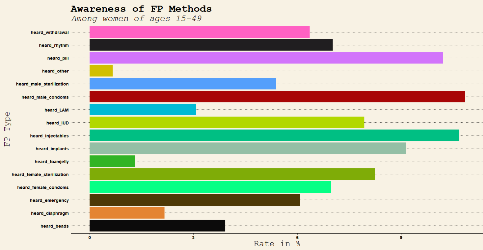
Overall Awareness Rates of Familiy planning Methods
Awareness<-FP_access %>%
  mutate(Aware=as.numeric(if_else(heard_female_sterilization|heard_male_sterilization|heard_implants|heard_IUD|
                                    heard_injectables|heard_pill|heard_emergency|heard_male_condoms|heard_female_condoms|
                                    heard_diaphragm|heard_foamjelly|heard_beads|heard_LAM|heard_rhythm|heard_withdrawal
                                  == "1", "1", "0")),
         IsAware=if_else(Aware=="1", "Yes","No")) %>%
  group_by(IsAware) %>%
  summarise(Count=n()) %>%
  mutate(Rate=round((Count/sum(Count))*100,2),
         Awareness_Rate=paste0(Rate, "%"),
         cumulative_ratio=cumsum(Rate),
         ration_min=c(0, head(cumulative_ratio,n=-1)),
         labelPosition=(cumulative_ratio+ration_min)/2,
         label=paste0(IsAware, ":", Awareness_Rate))

ggplot(Awareness,aes(ymax=cumulative_ratio, ymin=ration_min, xmax=4, xmin=3, fill=IsAware))+
  geom_rect()+
  scale_fill_manual(values = c(No = "#FFAFEEEE",
                               Yes = "#808080"))+
  geom_label(x=4.0,aes(y=labelPosition, label=label),size=6)+
  coord_polar(theta="y")+
  xlim(c(-1,4))+
  labs(title="FP Awareness Rate Among Women of Reproductive Age(15-49)")+
  theme_void()+
  theme(legend.position = "none")
Logistic Regression
From the Data, the study sought to build a model that can be used to assess factors that may lead a woman of reproductive age to use a family planning method. This model falls under the purview of classification since the response is a category data type.
Preping the data
Creating dummy variables. The response variable is generated from the current method column such that if a woman reports to be using a method then value 1 is used else 0. Other Dummy variables include IsReligious from religion column. Note that missing values and no responses are recorded as 0.
FP_Data<-PMA_DATA %>%
  mutate(age=as.numeric(age)) %>%
  filter(between (age,15,49)) %>%
  mutate(Aware=as.numeric(if_else(heard_female_sterilization|heard_male_sterilization|heard_implants|heard_IUD|
                                          heard_injectables|heard_pill|heard_emergency|heard_male_condoms|heard_female_condoms|
                                    heard_diaphragm|heard_foamjelly|heard_beads|heard_LAM|heard_rhythm|heard_withdrawal
                                  == "1", "1", "0")),
         IsAware=if_else(Aware=="1", "Yes","No")) %>%
  select(age,gender,current_method,religion, method_influences_pro,ever_birth, pregnant,
         marital_status, school, IsAware) %>%
  subset(gender==2)

FP_Data$current_method[FP_Data$current_method== "-99"]<-""
FP_Data$method_influences_pro[FP_Data$method_influences_pro== "-77"]<-""
FP_Data$pregnant[FP_Data$pregnant== "-88"]<-""
FP_Data$religion[FP_Data$religion== "-77"]<-""
FP_Data$religion[FP_Data$religion== "-88"]<-""
FP_Data$religion[FP_Data$religion== "-99"]<-""

FP_Data_Clean<-FP_Data %>%
  mutate(fp_use=as.numeric(if_else(current_method=="NA","0", "1")),
         been_influenced=as.numeric(if_else(method_influences_pro=="NA","0", "1")),
         IsReligious=as.numeric(if_else(religion=="NA","0","1")))

FP_Data_Clean$fp_use[is.na(FP_Data_Clean$fp_use)]<-0
FP_Data_Clean$been_influenced[is.na(FP_Data_Clean$been_influenced)]<-0
FP_Data_Clean$IsReligious[is.na(FP_Data_Clean$IsReligious)]<-0
FP_Data_Clean$pregnant[is.na(FP_Data_Clean$pregnant)]<-0
FP_Data_Clean$ever_birth[is.na(FP_Data_Clean$ever_birth)]<-0

Final_FP<-FP_Data_Clean %>%
  select(fp_use,age,IsReligious,marital_status,pregnant,been_influenced,ever_birth,school, IsAware) %>%
  mutate(fp_use=as.factor(fp_use),
         pregnant=as.numeric(pregnant))
Testing the claim whether awareness equals use
Awareness rates do not always indicate prevalence or preference rates. A two-sample t-test was used to compare difference between awareness and usage rates of FP method. The hypothesis was tested at 5% level of significance. Null hypothesis: μ1=μ2; awareness rate and usage rate of FP methods are equal. Alternative hypothesis: μ1≠μ2; awareness rate and usage rate of FP methods are not equal. Decision rule: p-value criteria, if the p-values are less than α (0.05), we reject the null hypothesis.
FP<-Final_FP %>%
  select(fp_use,IsAware) %>%
  mutate(Aware=as.numeric(if_else(IsAware=="Yes","1","0")),
         fp=as.numeric(if_else(fp_use=="1","1","0"))) %>%
  drop_na()
t.test(x=FP$Aware, y=FP$fp, alternative = "two.sided", conf.level = 0.95)
##
##  Welch Two Sample t-test
##
## data:  FP$Aware and FP$fp
## t = 80.443, df = 6515.7, p-value < 2.2e-16
## alternative hypothesis: true difference in means is not equal to 0
## 95 percent confidence interval:
##  0.5323172 0.5589096
## sample estimates:
## mean of x mean of y
## 0.9825236 0.4369102
From the output above, p-value of (2.2e-16) is less than (0.05). The null hypothesis is rejected We can conclude with 95% confidence that there exists sufficient statistical evidence that awareness rate and usage rate of FP methods among women of reproductive age is not the same.
Splitting the data
70-30 percent hold-out sample cross validation techniques was used to split the data into train and and test sets. This cross validation ratio sets up for the highest prediction accuracy.
splitratio<-sort(sample(nrow(Final_FP), nrow(Final_FP)*.7))
Final_FP_train<-Final_FP[splitratio,]
Final_FP_test<-Final_FP[-splitratio,]
Logistic Model 1
model1<-glm(fp_use~., family="binomial", data=Final_FP_train)
summary(model1)
##
## Call:
## glm(formula = fp_use ~ ., family = "binomial", data = Final_FP_train)
##
## Deviance Residuals:
##      Min        1Q    Median        3Q       Max
## -2.44171  -0.00006  -0.00003   0.35435   1.05772
##
## Coefficients:
##                   Estimate Std. Error z value Pr(>|z|)
## (Intercept)     -2.076e+01  2.017e+03  -0.010   0.9918
## age              7.032e-03  1.267e-02   0.555   0.5789
## IsReligious     -3.619e-01  2.312e-01  -1.565   0.1175
## marital_status  -1.323e-01  6.646e-02  -1.990   0.0466 *
## pregnant        -2.150e+01  8.701e+02  -0.025   0.9803
## been_influenced  2.240e+01  3.766e+02   0.059   0.9526
## ever_birth       1.378e+00  2.812e-01   4.900 9.58e-07 ***
## school          -3.844e-02  6.488e-02  -0.592   0.5535
## IsAwareYes      -2.634e-01  2.052e+03   0.000   0.9999
## ---
## Signif. codes:  0 '***' 0.001 '**' 0.01 '*' 0.05 '.' 0.1 ' ' 1
##
## (Dispersion parameter for binomial family taken to be 1)
##
##     Null deviance: 5453.9  on 3971  degrees of freedom
## Residual deviance: 1098.9  on 3963  degrees of freedom
##   (71 observations deleted due to missingness)
## AIC: 1116.9
##
## Number of Fisher Scoring iterations: 19
Only one factor was significant in the model and therefore the model was doing a bad job.
Logistic model 2
Transforming age into logs to try and check for significance.
model2<-glm(fp_use~school+ever_birth+marital_status+log(age), family="binomial", data=Final_FP_train)
summary(model2)
##
## Call:
## glm(formula = fp_use ~ school + ever_birth + marital_status +
##     log(age), family = "binomial", data = Final_FP_train)
##
## Deviance Residuals:
##     Min       1Q   Median       3Q      Max
## -1.7968  -1.0971  -0.3661   1.0793   2.3579
##
## Coefficients:
##                Estimate Std. Error z value Pr(>|z|)
## (Intercept)    -1.71649    0.47985  -3.577 0.000347 ***
## school          0.29349    0.02866  10.240  < 2e-16 ***
## ever_birth      2.10460    0.13942  15.095  < 2e-16 ***
## marital_status -0.20660    0.02737  -7.548 4.41e-14 ***
## log(age)       -0.07879    0.14494  -0.544 0.586745
## ---
## Signif. codes:  0 '***' 0.001 '**' 0.01 '*' 0.05 '.' 0.1 ' ' 1
##
## (Dispersion parameter for binomial family taken to be 1)
##
##     Null deviance: 5491.9  on 4002  degrees of freedom
## Residual deviance: 4493.7  on 3998  degrees of freedom
##   (40 observations deleted due to missingness)
## AIC: 4503.7
##
## Number of Fisher Scoring iterations: 4
This model was a little better than the first one as illustrated by more significant variables.
Logistic Model 3
model3<-glm(fp_use~school+ever_birth+marital_status+IsReligious+IsAware, family="binomial", data=Final_FP_train)
summary(model3)
##
## Call:
## glm(formula = fp_use ~ school + ever_birth + marital_status +
##     IsReligious + IsAware, family = "binomial", data = Final_FP_train)
##
## Deviance Residuals:
##     Min       1Q   Median       3Q      Max
## -1.7888  -1.0176  -0.3827   1.0624   2.4568
##
## Coefficients:
##                 Estimate Std. Error z value Pr(>|z|)
## (Intercept)    -17.28191  254.76040  -0.068 0.945916
## school           0.27438    0.02888   9.501  < 2e-16 ***
## ever_birth       2.17366    0.13259  16.394  < 2e-16 ***
## marital_status  -0.17005    0.02880  -5.904 3.55e-09 ***
## IsReligious     -0.39059    0.10662  -3.663 0.000249 ***
## IsAwareYes      15.28067  254.76037   0.060 0.952171
## ---
## Signif. codes:  0 '***' 0.001 '**' 0.01 '*' 0.05 '.' 0.1 ' ' 1
##
## (Dispersion parameter for binomial family taken to be 1)
##
##     Null deviance: 5491.9  on 4002  degrees of freedom
## Residual deviance: 4444.7  on 3997  degrees of freedom
##   (40 observations deleted due to missingness)
## AIC: 4456.7
##
## Number of Fisher Scoring iterations: 15
tidy(model3)
## # A tibble: 6 × 5
##   term           estimate std.error statistic  p.value
##   <chr>             <dbl>     <dbl>     <dbl>    <dbl>
## 1 (Intercept)     -17.3    255.       -0.0678 9.46e- 1
## 2 school            0.274    0.0289    9.50   2.07e-21
## 3 ever_birth        2.17     0.133    16.4    2.12e-60
## 4 marital_status   -0.170    0.0288   -5.90   3.55e- 9
## 5 IsReligious      -0.391    0.107    -3.66   2.49e- 4
## 6 IsAwareYes       15.3    255.        0.0600 9.52e- 1
Since all predictors chosen indicated significant p-values and the Mac Fadden’s statistic of 0.237 lies between 0.2 and 0.4, the model is selected as its meets the requirements of a good model.
Tabulating model 3 parameters in HTML format and generating McFadden’s statistic
The packages below help render beautiful output of logistic model parameters including the parameters’ odds ratios,their CI’s, p-values as well as McFadden’s statistic
library(sjPlot)
library(sjmisc)
library(sjlabelled)
tab_model(model3)
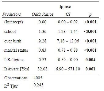
Explanation of the model parameters.
school This variable was an ordinal variable explaining the current education level of the respondent. It was recorded as none, primary, secondary, tertiary. Given a unit increase in the level of education, the odds of a woman using a family planning method increases by 1.36. This information is significant in that it tells us education is very influential in whether a woman uses a FP method.
ever birth This variable recorded whether a woman had given birth before. A woman who had given birth was 9.28 times more likely to use a family planning method. Probable reasons could be;
- May be the pregnancy was accidental and was the woman was much more keen to avoid another.
- The economic conditions were not suitable for a woman to raise another child.
- The woman may have been satisfied with the current number of children she has and was not planning of having others in the near future.
IsReligious This variable was a dummy variable generated from the religion type of the respondents. Religious respondents were 0.73 times more likely to use a family planning method. This could be attributed to the fact that religious leader are among the modern day propagators of family planning and even allow education of family planning in their religious institutions.
Prediction and Model Assessment
1. Using Performance Metrics Classification models can me assesd using various metrics. They include;
- Confusion Matrix
- Sensitivity
- Specificity
- Accuracy There are more metrics which you can learn form the link below https://www.analyticsvidhya.com/blog/2021/07/metrics-to-evaluate-your-classification-model-to-take-the-right-decisions/#
library(caret)
prediction1<- predict(model3, Final_FP_test, type='response')
prediction2<- predict(model3, Final_FP_test, type='link')
head(prediction1)
##         1         2         3         4         5         6
## 0.1162593 0.0706267 0.0706267 0.2893870 0.5687495 0.1162593
predicted_data<- as.factor((ifelse(prediction1>=0.5, "1", "0")))
print(confusionMatrix(predicted_data, Final_FP_test$fp_use))
## Confusion Matrix and Statistics
##
##           Reference
## Prediction   0   1
##          0 620 135
##          1 361 603
##
##                Accuracy : 0.7115
##                  95% CI : (0.6894, 0.7328)
##     No Information Rate : 0.5707
##     P-Value [Acc > NIR] : < 2.2e-16
##
##                   Kappa : 0.4327
##
##  Mcnemar's Test P-Value : < 2.2e-16
##
##             Sensitivity : 0.6320
##             Specificity : 0.8171
##          Pos Pred Value : 0.8212
##          Neg Pred Value : 0.6255
##              Prevalence : 0.5707
##          Detection Rate : 0.3607
##    Detection Prevalence : 0.4392
##       Balanced Accuracy : 0.7245
##
##        'Positive' Class : 0
##
71.46% of the time, this model predicts an observation correctly with 95% CI : (0.6926, 0.7359) and a precision of 64.17%. Sensitivity (Recall) tells us how many predictions are actual positives. The model has a recall value of 65.7%. Specificity is the proportion of actual negatives. The model has a specificity of 78.86%
2. Mc Nemar Test Testing for significant difference between the actual and predicted values Hypothesis 𝐻0: There is no difference, i.e. 𝐻0: 𝑝1= 𝑝2 against, 𝐻1: There is a difference, i.e. 𝐻0: 𝑝1 ≠ 𝑝2.
The model metric gave a p-value of (1.119e-14) which is less than alpha (0.05) therefore the null hypothesis is rejected.
3. Is the model a best fit Chi-square test is used to assess this.
with(model3,pchisq(null.deviance-deviance,df.null-df.residual,lower.tail=F))
## [1] 3.703714e-224
The Model is statistically significant.
4. ROC Curve and AUC Score
library(pROC)
simple_roc <- function(labels, scores){
  labels <- labels[order(scores, decreasing=TRUE)]
  data.frame(TPR=cumsum(labels)/sum(labels), FPR=cumsum(!labels)/sum(!labels), labels)
}
plot(roc(Final_FP_test$fp_use, prediction2), main="True Positive Rate vs False Positive Rate", print.auc=TRUE)

simp_roc <- simple_roc(Final_FP_test$fp_use=="TRUE",prediction2)
with(simp_roc, lines(1 - FPR, TPR, col="blue", lty=2))
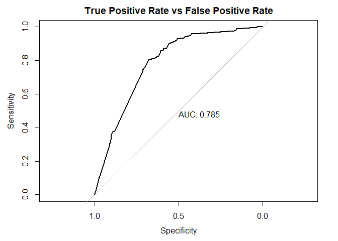 The AUC Score is 0.773 This fairly good.