Introduction to Factorial Experiments

This is the last section on my series of the various designs of experiments using R. These designs are what are commonly referred to as one factor at a time experiment. Make sure to read the previous post on CRD and RBD experiments.

What are Factorial Experiments?

Many experiments involve the study of the effects of two or more factors. In general, factorial designs are most efficient for this type of experiment. By a factorial design, we mean that in each complete trial or replicate of the experiment all possible combinations of the levels of the factors are investigated. For example, if there are a levels of factor A and b levels of factor B, each replicate contains all ab treatment combinations. When factors are arranged in a factorial design, they are often said to be crossed. The effect of a factor is defined to be the change in response produced by a change in the level of the factor. This is frequently called a main effect because it refers to the primary factors of interest in the experiment. (Montgomery, 2012)

Factorial experiments allow us to analyze the effects of factors simultaneously. The most common are the 2 factor factorials also known as the 2k experiments, where k can take the values (2,3,…).

Advantages of Factorial Experiments Over One Factor at a Time Experiments

They are more efficient in that they provide more information at lower or similar cost as compared to one factor at a time experiments.
Allows a researcher to study how the factors interact within themselves.

Disadvantages

Some experiments may be cumbersome to compute mathematically especially if they involve numerous factors.
Some information may be lost during the design of a factorial experiment. This is a phenomenon known as confounding.

I will not get into the manual derivations of how to solve factorial experiments but, I will however attach some reference where one can get more information about it.

Factorial Designs Using R

To perform these experiments, we will use the DoeBioresearch package. Additionally, I have partnered with two friends; who are both microbiologists and have allowed me to use their experimental data for this illustration.

Example 1

In this example, my friend Joseah Lang’at check out his LinkedIn profile was performing an experiment SENSITIVITY OF *Staphylococcus aureus AND Escherichia coli TO Zingiber officinale AND Allium sativum EXTRACTS*. In simpler terms, the title of the experiment was assessing how sensitive the two bacteria were to extracts of ginger and garlic.

The main objectives of the experiment were; To determine the sensitivity of Staphylococcus aureus and Escherichia coli to Zingiber officinale and Allium sativum.

The data contained the following; Concentration. This represents levels of distilled water. (1,2,3) representing (0%, 50%, 25%) distilled water respectively. Treatments. There Value. This is the zone of inhibition recorded in the experiment. The values are in centimeters.

Loading the data and required packages

library(doebioresearch)
library(readxl)
sensitivity_data <- read_excel("SensitivityData.xlsx", 
    sheet = "saureus")

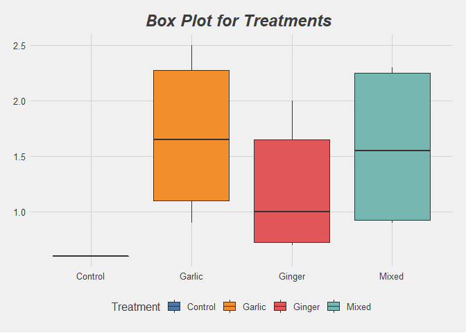
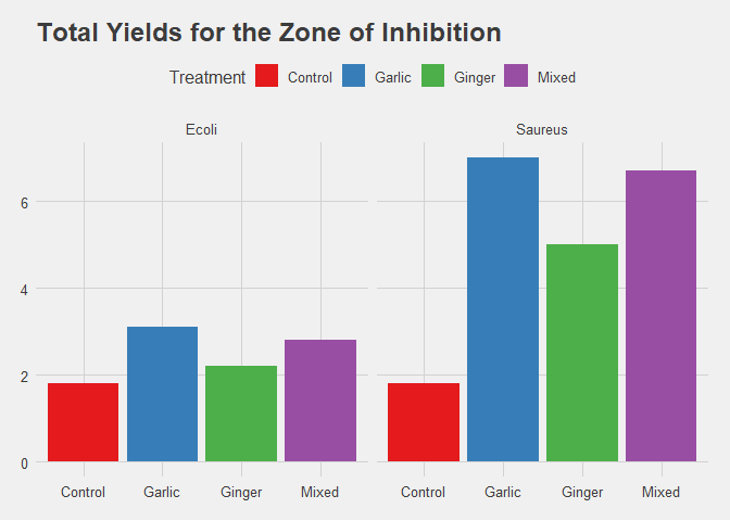
Some Visualizations

library(ggplot2)
library(ggthemes)
ggplot(sensitivity_data) +
  aes(x = Treatment, y = Value, fill = Treatment) +
  geom_boxplot(shape = "circle") +
  scale_fill_hue(direction = 1) +
  labs(title = "Box Plot for Treatments ") +
  scale_fill_tableau()+
  ggthemes::theme_fivethirtyeight() +
  theme(plot.title = element_text(face = "bold.italic",hjust = 0.5))

ggplot(sensitivity_data) +
  aes(x = Treatment, fill = Treatment, weight = Value) +
  geom_bar() +
  scale_fill_brewer(palette = "Set1", direction = 1) +
  labs(y = "Yield",
    title = "Total Yields for the Zone of Inhibition") +
  ggthemes::theme_fivethirtyeight() +
  theme(legend.position = "top") +
  facet_wrap(vars(Bacteria))

ggplot(sensitivity_data) +
  aes(x = Bacteria, y = Value, fill = Bacteria) +
  geom_boxplot(shape = "circle") +
  scale_fill_hue(direction = 1) +
  labs(title = "Boxplot for the Bacteria") +
  theme_minimal() +
  scale_fill_tableau()+
  theme(plot.title = element_text(face = "bold.italic",hjust = 0.5))

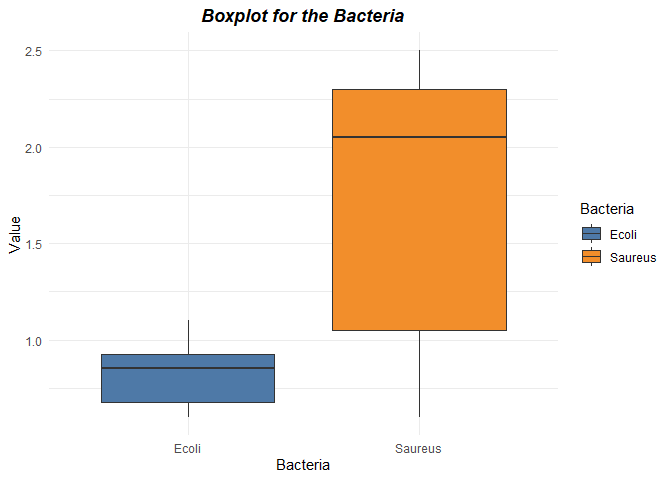
No presence of Outliers from the plots above.

Running a factorial experiment.

To analyze the significance of the factors in the experiment, a 2^2 factorial experiment was chosen. This experiment was carried out at 5% level of significance. The Least Significant Difference was used to check on the of the differences between statistically significant groups. The two factors are Bacteria and Treatments. Concentration was taken as the blocking/replication factor.

Hypotheses

Treatments (Factor A) Null: Anti-microbial activity between the treatments are equal. Alternative: At least one of the treatments has a different Anti-microbial activity.
Bacteria (Factor B) Null: S.aureus and E.coli have similar sensitivity effect on the extracts. Alternative: S.aureus and E.coli do not have similar sensitivity effect on the extracts.
Blocks (Concetration of Distilled Water) Null: Blocks have similar effect Alternative: At least one is different

Decision Rule If p-value is less than alpha(0.05) we reject the null hypothesis.

frbd2fact(sensitivity_data[3], sensitivity_data$Concentration,
                  sensitivity_data$Treatment,sensitivity_data$Bacteria,1)

## $Value
## $Value[[1]]
## Analysis of Variance Table
## 
## Response: dependent.var
##                   Df Sum Sq Mean Sq  F value    Pr(>F)    
## replicationvector  2 0.1408  0.0704   3.0888   0.07741 .  
## fact.A             3 4.3367  1.4456  63.4082 2.167e-08 ***
## fact.B             1 4.6817  4.6817 205.3577 9.299e-10 ***
## fact.A:fact.B      3 1.6950  0.5650  24.7833 7.315e-06 ***
## Residuals         14 0.3192  0.0228                       
## ---
## Signif. codes:  0 '***' 0.001 '**' 0.01 '*' 0.05 '.' 0.1 ' ' 1
## 
## $Value[[2]]
## [1] "R Square 0.971"
## 
## $Value[[3]]
## [1] "SEm of A: 0.062 , SEd of A: 0.087 , SEm of B: 0.044 , SEd of B 0.062 , SEm of AB: 0.087 , SEd of AB: 0.123"
## 
## $Value[[4]]
## 
##  Shapiro-Wilk normality test
## 
## data:  model$residuals
## W = 0.89877, p-value = 0.02027
## 
## $Value[[5]]
## [1] "Normality assumption is violated"
## 
## $Value[[6]]
## [1] "The means of one or more levels of first factor are not same, so go for multiple comparison test"
## 
## $Value[[7]]
## $Value[[7]][[1]]
##      MSerror Df     Mean       CV  t.value       LSD
##   0.02279762 14 1.266667 11.92017 2.144787 0.1869684
## 
## $Value[[7]][[2]]
##         dependent.var groups
## Garlic       1.683333      a
## Mixed        1.583333      a
## Ginger       1.200000      b
## Control      0.600000      c
## 
## $Value[[8]]
## [1] "The means of one or more levels of second factor are not same, so go for multiple comparison test"
## 
## $Value[[9]]
## $Value[[9]][[1]]
##      MSerror Df     Mean       CV  t.value       LSD
##   0.02279762 14 1.266667 11.92017 2.144787 0.1322066
## 
## $Value[[9]][[2]]
##         dependent.var groups
## Saureus      1.708333      a
## Ecoli        0.825000      b
## 
## $Value[[10]]
## [1] "The means of levels of interaction between two factors are not same, so go for multiple comparison test"
## 
## $Value[[11]]
## $Value[[11]][[1]]
##      MSerror Df     Mean       CV  t.value       LSD
##   0.02279762 14 1.266667 11.92017 2.144787 0.2644133
## 
## $Value[[11]][[2]]
##                 dependent.var groups
## Garlic:Saureus      2.3333333      a
## Mixed:Saureus       2.2333333      a
## Ginger:Saureus      1.6666667      b
## Garlic:Ecoli        1.0333333      c
## Mixed:Ecoli         0.9333333     cd
## Ginger:Ecoli        0.7333333     de
## Control:Ecoli       0.6000000      e
## Control:Saureus     0.6000000      e

Result Interpretation

ANOVA TABLE
Are the concentration (Block) significant?

The test returned a p-value of (0.07741) for the blocks. This is greater than 0.05. The decision is therefore fail to reject the null hypothesis and conclude that with 95% confidence, the concentration effects of distilled water are statistically insignificant to the experimental yield.

Are the Effects of the Extracts Significant?

A p-value of (2.167e-08) was returned by the test. This is less than 0.05. The null hypothesis is rejected and conclude that with 95% confidence, that the effects of the plant extracts differ significantly.

Are the Effects of the Bacteria Significant?

The p-value (9.299e-10) is less than 0.05. We therefore reject the null hypothesis and conclude that with 95% confidence, that the effects of the bacteria differ significantly. Main effects are significant

Are the Two-Factor Interaction Effects Significant?

The p-value (9.299e-10) is less than 0.05. We therefore reject the null hypothesis and conclude that with 95% confidence, that the interaction effects are statistically significant.

R Square 0.971, indicates that this model explains 97.1% variability. This is a good result.

Multiple Comparison Tests Having rejected the null hypothesis in for main effects and interactions, the LSD test was used to test and select the effects with the most significance.

Treatments

Of the 4 treatments, no statistical difference exists between Garlic and Mixed. These two offer the highest anti-microbial activity. When compared across the treatments, Garlic and Mixed differed significantly from ginger and control.

Bacteria

S.aureus had the highest sensitivity as compared to E.coli with a mean of 1.708 as compared to 0.825 for E.coli.

Interaction Effects

The interaction Garlic:S.aureus and Mixed:S.aureus offered the highest yield and there was no statistical differences between these interactions.

In chronological order, the interaction effects were as follows;

Garlic:Saureus and Mixed:Saureus
Ginger:Saureus
Garlic:Ecoli
Mixed:Ecoli
Ginger:Ecoli
Control:Ecoli
7.Control:Saureus

To conclude this experiment, an interaction plot was used to visualize the presecence of interaction between the two factors.

Checking for interaction within the data

We use the interaction.plot function to check on interaction between the two factors; Bacteria and treatment

interaction.plot(x.factor=sensitivity_data$Bacteria,
                 trace.factor=sensitivity_data$Treatment,
                 response=sensitivity_data$Value,
                 type="b", 
                 main="Interaction Between Bacteria and Plant Extracts",
                 xlab="Bacteria",
                 ylab = "Zone of Inhibition in cm",
                 col = c("red","blue", "green", "black"),
                 lwd=2,
                 trace.label = "Extract") 

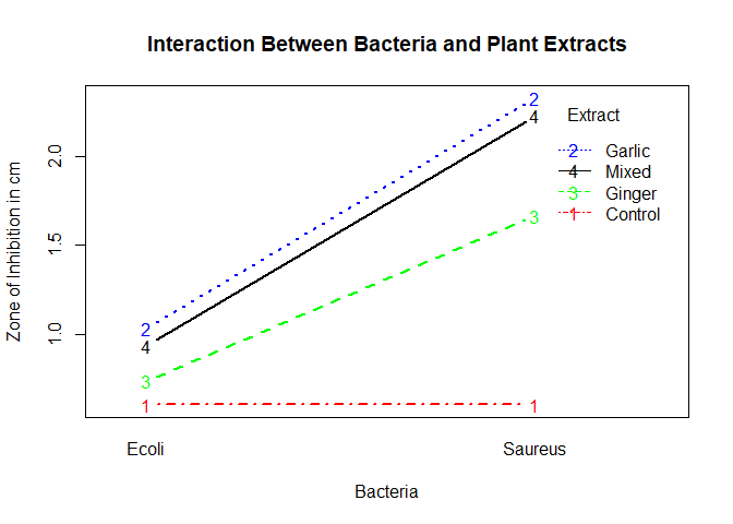From the plot, Garlic has the highest antimicrobial activity followed by mixed then ginger and finally control. S.aureus has higher sensitivity as compared to E.coli. However, we can not conclude that there is presence of interaction between the two factors. Additionally, there is an increase in the sensitivity of the bacteria as you move from E.coli to S.aureus

Example 2

In this example, my friend Gideon check out his [LinkedIn page]9(https://www.linkedin.com/in/steve-gideons-b390761a1/) was performing an experiment title Prevalence of Bovine Mastitis and their Anti-microbial Susceptibility Profile in London Ward, Nakuru County The objectives of the research were to determine the prevelence of mastitis, identify the most prevalent bacteria causing mastitis and determine their antimicrobial susceptibility profile.

Bovine Mastitis is an inflammatory response of the udder tissue in mammary gland caused due to physical trauma or microorganism infections. It is considered the most common disease leading to economic loss in dairy industries due to reduced yield and poor quality of milk. (Henriques and Gomes, 2016)

In summary, the research sought to investigate the most dominant bacteria that causes bovine mastitis and which type of mastitis diagnosis is the most prevalent. Finally, the research looked into some common antibiotics to understand which one was effective against what type of bovine mastitis. The study was conducted in London ward and a sample of 15 cows were randomly selected and milk samples drawn from them. Laboratory tests were performed and respective zone of inhibition recorded.

Loading the Data and some required packages

library(readxl)
library(dplyr)
library(tidyr)
library(knitr)
library(ggplot2)
library(ggthemes)
Mastistis <- read_excel("MastitisData.xlsx", 
    sheet = "Sheet1", col_types = c("text", 
        "text", "text", "text", "text", "text", 
        "numeric"))

The data contained the following variables;

Specimen_No
Breed - Type of cow; Friesian, Jersey or Ayshire
Quarters - Cow’s tits. Front Left (FL), Front Right, Back Left, Back Right
Isolates - Bacteria identified
Diagnosis - Type of mastitis
Sensitivity_test - Antibiotic administered
Yield - Zone of inhibition recorded in millimeters.

Some Exploratory Data Analysis

Zone of Inhibition by Breed

Breed_Summary<-Mastistis %>% 
  group_by(Breed) %>%
  drop_na() %>% 
  summarise(Count=n(),
            Average_Zone= mean(Yield),
            SD=sd(Yield),
            SE=SD/Count,
            LCL=round(Average_Zone-(1.96*SE),2),
            UCL=round(Average_Zone+(1.96*SE),2),
            Zone_Mean_95Pct_CI=paste("(", LCL ," , ", UCL, ")" ))

kable(Breed_Summary %>% 
        select(-c(LCL,UCL, SE)))

Breed	Count	Average_Zone	SD	Zone_Mean_95Pct_CI
Ayshire	80	19.65000	5.388924	( 19.52 , 19.78 )
Fresian	168	19.10119	5.439531	( 19.04 , 19.16 )
Jersey	56	19.73214	4.669012	( 19.57 , 19.9 )

Aggregation by Isolates

Isolate<-Mastistis %>% 
  group_by(Isolates) %>% 
  summarise(Count=n()) %>% 
  mutate(Pct=(round(Count/sum(Count),2)*100),
         Isolate_int=c("Ent","E.coli", "Klebsiella", "No_Isolate", "Pseudomonas",
                       "Staphylococcus"),
         Rate=paste0(Pct, "%"),
         cumulative_ratio=cumsum(Pct),
         ration_min=c(0, head(cumulative_ratio,n=-1)),
         labelPosition=(cumulative_ratio+ration_min)/2,
         label=paste0(Isolate_int, ":", Rate))

ggplot(Isolate,aes(ymax=cumulative_ratio, ymin=ration_min, xmax=4, xmin=3, 
                   fill=Isolate_int))+
  geom_rect()+
  scale_fill_manual(values = c(Ent = "red", 
                               E.coli = "orange",
                               Klebsiella= "green",
                               No_Isolate = "blue",
                               Pseudomona = "yellow",
                               Staphylococcus= "purple"))+
  geom_label(x=2.6,aes(y=labelPosition, label=label),size=6)+
  coord_polar(theta="y")+
  xlim(c(-1,4))+
  labs(title="ISOLATES",
       subtitle = ("Enterecoccus, E.coli, Klebsiella, No_Isolate, Pseudomonas,
                       Staphylococcus"))+
  theme(plot.title = element_text(face = "bold.italic",hjust = 0.5))+
  theme_void()+
  theme(legend.position = "none")

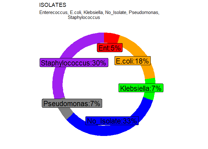33% of the samples showed no isolate. This is a warying statistic since it implies that the prevalence rate of Bovine mastitis is at 67% which is relatively high.

Dropping values with No isolates

no_isolate<-Mastistis %>% 
  filter(Isolates=="No isolate")
Mastistis_clean<-Mastistis[!Mastistis$Isolates=="No isolate",]

Mastistis_clean <-Mastistis_clean %>% 
  mutate(Breed=as.factor(Breed),
         Quarters=as.factor(Quarters),
         Isolates=as.factor(Isolates),
         Diagnosis=as.factor(Diagnosis),
         Yield=as.numeric(Yield))

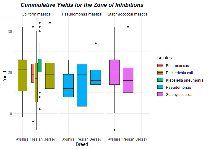
Cummulative Yields for the Zone of Inhibitions

ggplot(Mastistis_clean) +
  aes(x = Breed, y = Yield, fill = Isolates) +
  geom_boxplot(shape = "circle") +
  scale_fill_hue(direction = 1) +
  labs(title = "Cummulative Yields for the Zone of Inhibitions") +
  theme_minimal() +
  theme(plot.title = element_text(face = "bold.italic",hjust = 0.5)) +
  facet_wrap(vars(Diagnosis))

Analysis of Diagnosis and the Anti-microbial Agents

To test for the significance in the mean differences, 3k factorial experiment was chosen.The Least Significant Difference was used to check on the of the differences between statistically significant groups. The three factors are Diagnosis, Sensitivity and Breed. Quarters was taken as the blocking/replication factor.

Hypotheses

Diagnosis (Factor A) Null: The diagnosis are similar in effect. Alternative: At least one of the diagnosis has a different effect.
Sensitivity (Factor B) These are the drugs subjected to the pathogens associated with mastitis. Null: The Sensitivity have similar effects. Alternative: At least one of the Sensitivity is different.
Breed (Factor C) Null: The breeds have similar effects. Alternative: At least one of the breeds is different.
Blocks Null: Blocks have similar effect. Alternative: At least one is different.
Interaction effects Null: Two and three factor interactions have similar effect. Alternative: At least one the interaction sets is different.

Decision rule p-value criteria. If p-value is less than alpha (0.05), the null hypothesis is rejected.

library(doebioresearch)
frbd3fact(Mastistis_clean[7], Mastistis_clean$Quarters, Mastistis_clean$Diagnosis,
          Mastistis_clean$Sensitivity_test, Mastistis_clean$Breed, 1)

## $Yield
## $Yield[[1]]
## Analysis of Variance Table
## 
## Response: dependent.var
##                       Df Sum Sq Mean Sq F value    Pr(>F)    
## replicationvector      9  179.2  19.909  0.9633  0.471279    
## fact.A                 2  220.9 110.441  5.3434  0.005388 ** 
## fact.B                 7 1405.0 200.720  9.7113 1.366e-10 ***
## fact.C                 2    1.5   0.728  0.0352  0.965412    
## fact.A:fact.B         14  589.4  42.098  2.0368  0.016189 *  
## fact.A:fact.C          3   41.6  13.854  0.6703  0.571066    
## fact.B:fact.C         14  729.8  52.129  2.5221  0.002284 ** 
## fact.A:fact.B:fact.C  21  518.4  24.688  1.1945  0.256982    
## Residuals            231 4774.5  20.669                      
## ---
## Signif. codes:  0 '***' 0.001 '**' 0.01 '*' 0.05 '.' 0.1 ' ' 1
## 
## $Yield[[2]]
## [1] "R Square 0.436"
## 
## $Yield[[3]]
## [1] "SEm of A: 0.293 , SEd of A: 0.415 , SEm of B: 0.479 , SEd of B 0.678 , SEm of C: 0.293 , SEd of C: 0.415 , SEm of AB: 0.83 , SEd of AB: 1.174 , SEm of AC: 0.508 , SEd of AC: 0.719 , SEm of BC: 0.83 , SEd of BC: 1.174 , SEm of ABC: 1.438 , SEd of ABC: 2.033"
## 
## $Yield[[4]]
## 
##  Shapiro-Wilk normality test
## 
## data:  model$residuals
## W = 0.98536, p-value = 0.003476
## 
## 
## $Yield[[5]]
## [1] "Normality assumption is violated"
## 
## $Yield[[6]]
## [1] "The means of one or more levels of factor A are not same, so go for multiple comparison test"
## 
## $Yield[[7]]
## $Yield[[7]][[1]]
##    MSerror  Df     Mean       CV
##   20.66862 231 19.36184 23.48059
## 
## $Yield[[7]][[2]]
##                         dependent.var groups
## Coliform mastitis            20.05882      a
## Staphylococcal mastitis      18.92647      b
## Pseudomonas mastitis         18.25000      b
## 
## 
## $Yield[[8]]
## [1] "The means of one or more levels of factor B are not same, so go for multiple comparison test"
## 
## $Yield[[9]]
## $Yield[[9]][[1]]
##    MSerror  Df     Mean       CV  t.value      LSD
##   20.66862 231 19.36184 23.48059 1.970287 2.054983
## 
## $Yield[[9]][[2]]
##               dependent.var groups
## Gentamycin         23.31579      a
## Neomycin           20.68421      b
## Cefalexin          20.57895      b
## Streptomycin       19.60526     bc
## Tetracycline       18.73684     bc
## Kanamycin          18.71053     bc
## Penicillin         17.71053      c
## Cotrimoxazole      15.55263      d
## 
## 
## $Yield[[10]]
## [1] "All the factor C level means are same so dont go for any multiple comparison test"
## 
## $Yield[[11]]
## $Yield[[11]][[1]]
##    MSerror  Df     Mean       CV
##   20.66862 231 19.36184 23.48059
## 
## $Yield[[11]][[2]]
##         dependent.var groups
## Jersey       19.73214      a
## Ayshire      19.65000      a
## Fresian      19.10119      a
## 
## $Yield[[12]]
## [1] "The means of levels of interaction between A and B factors are not same, so go for multiple comparison test"
## 
## $Yield[[13]]
## $Yield[[13]][[1]]
##    MSerror  Df     Mean       CV
##   20.66862 231 19.36184 23.48059
## 
## $Yield[[13]][[2]]
##                                       dependent.var groups
## Coliform mastitis:Gentamycin               24.05882      a
## Staphylococcal mastitis:Gentamycin         23.70588     ab
## Coliform mastitis:Tetracycline             21.64706    abc
## Coliform mastitis:Cefalexin                21.58824    abc
## Pseudomonas mastitis:Neomycin              21.50000   abcd
## Staphylococcal mastitis:Neomycin           20.76471    bcd
## Pseudomonas mastitis:Kanamycin             20.75000   bcde
## Coliform mastitis:Streptomycin             20.47059    cde
## Staphylococcal mastitis:Kanamycin          20.47059    cde
## Coliform mastitis:Neomycin                 20.41176    cde
## Staphylococcal mastitis:Cefalexin          19.88235    cde
## Pseudomonas mastitis:Streptomycin          19.75000    cde
## Pseudomonas mastitis:Cefalexin             19.25000   cdef
## Coliform mastitis:Penicillin               18.70588   cdef
## Staphylococcal mastitis:Streptomycin       18.70588   cdef
## Pseudomonas mastitis:Gentamycin            18.50000  cdefg
## Pseudomonas mastitis:Tetracycline          17.75000  cdefg
## Coliform mastitis:Cotrimoxazole            17.11765   defg
## Staphylococcal mastitis:Penicillin         17.05882   defg
## Coliform mastitis:Kanamycin                16.47059    efg
## Pseudomonas mastitis:Penicillin            16.25000    efg
## Staphylococcal mastitis:Tetracycline       16.05882    efg
## Staphylococcal mastitis:Cotrimoxazole      14.76471     fg
## Pseudomonas mastitis:Cotrimoxazole         12.25000      g
## 
## 
## $Yield[[14]]
## [1] "The means of levels of interaction between B and C factors are not same, so go for multiple comparison test"
## 
## $Yield[[15]]
## $Yield[[15]][[1]]
##    MSerror  Df     Mean       CV
##   20.66862 231 19.36184 23.48059
## 
## $Yield[[15]][[2]]
##                       dependent.var groups
## Tetracycline:Jersey        26.14286      a
## Gentamycin:Ayshire         24.80000     ab
## Gentamycin:Fresian         23.23810    abc
## Cefalexin:Ayshire          21.50000    bcd
## Gentamycin:Jersey          21.42857    bcd
## Neomycin:Jersey            21.28571    bcd
## Streptomycin:Fresian       21.04762     cd
## Neomycin:Fresian           20.90476     cd
## Cefalexin:Fresian          20.85714     cd
## Kanamycin:Ayshire          20.30000     cd
## Neomycin:Ayshire           19.80000    cde
## Penicillin:Jersey          19.57143   cdef
## Kanamycin:Fresian          19.00000    def
## Tetracycline:Ayshire       18.90000    def
## Cefalexin:Jersey           18.42857   defg
## Streptomycin:Ayshire       18.30000   defg
## Cotrimoxazole:Jersey       18.28571   defg
## Penicillin:Ayshire         18.20000   defg
## Streptomycin:Jersey        17.14286   defg
## Penicillin:Fresian         16.85714    efg
## Tetracycline:Fresian       16.19048     fg
## Kanamycin:Jersey           15.57143     fg
## Cotrimoxazole:Ayshire      15.40000     fg
## Cotrimoxazole:Fresian      14.71429      g
## 
## 
## $Yield[[16]]
## [1] "The means of levels of interaction between A and C factors are same so dont go for any multiple comparison test"
## 
## $Yield[[17]]
## $Yield[[17]][[1]]
##    MSerror  Df     Mean       CV
##   20.66862 231 19.36184 23.48059
## 
## $Yield[[17]][[2]]
##                                 dependent.var groups
## Coliform mastitis:Fresian            20.30556      a
## Staphylococcal mastitis:Ayshire      20.01786      a
## Coliform mastitis:Jersey             19.83333      a
## Coliform mastitis:Ayshire            19.62500     ab
## Pseudomonas mastitis:Jersey          19.12500     ab
## Pseudomonas mastitis:Fresian         18.37500     ab
## Staphylococcal mastitis:Fresian      18.16250      b
## Pseudomonas mastitis:Ayshire         17.12500      b
## 
## 
## $Yield[[18]]
## [1] "The means of levels of interaction between all the three factors ABC are same so dont go for any multiple comparison test"
## 
## $Yield[[19]]
## $Yield[[19]][[1]]
##    MSerror  Df     Mean       CV
##   20.66862 231 19.36184 23.48059
## 
## $Yield[[19]][[2]]
##                                               dependent.var groups
## Pseudomonas mastitis:Neomycin:Fresian              27.00000      a
## Pseudomonas mastitis:Tetracycline:Jersey           27.00000     ab
## Coliform mastitis:Tetracycline:Jersey              26.00000     ab
## Staphylococcal mastitis:Gentamycin:Ayshire         25.57143     ab
## Coliform mastitis:Gentamycin:Fresian               25.44444     ab
## Coliform mastitis:Cefalexin:Ayshire                25.00000     ab
## Coliform mastitis:Gentamycin:Ayshire               24.00000    abc
## Pseudomonas mastitis:Kanamycin:Ayshire             23.00000   abcd
## Coliform mastitis:Cefalexin:Fresian                22.77778   abcd
## Coliform mastitis:Streptomycin:Fresian             22.66667   abcd
## Coliform mastitis:Penicillin:Ayshire               22.50000   abcd
## Staphylococcal mastitis:Gentamycin:Fresian         22.40000   abcd
## Coliform mastitis:Gentamycin:Jersey                22.00000   abcd
## Pseudomonas mastitis:Penicillin:Jersey             22.00000  abcde
## Coliform mastitis:Neomycin:Jersey                  21.83333  abcde
## Pseudomonas mastitis:Cefalexin:Fresian             21.50000  abcde
## Pseudomonas mastitis:Streptomycin:Fresian          21.50000  abcde
## Staphylococcal mastitis:Cefalexin:Ayshire          21.14286  abcde
## Pseudomonas mastitis:Gentamycin:Ayshire            21.00000 abcdef
## Staphylococcal mastitis:Neomycin:Fresian           21.00000 abcdef
## Staphylococcal mastitis:Tetracycline:Ayshire       21.00000 abcdef
## Staphylococcal mastitis:Kanamycin:Ayshire          20.57143 abcdef
## Coliform mastitis:Neomycin:Ayshire                 20.50000 abcdef
## Coliform mastitis:Streptomycin:Ayshire             20.50000 abcdef
## Coliform mastitis:Tetracycline:Fresian             20.44444 abcdef
## Staphylococcal mastitis:Neomycin:Ayshire           20.42857 abcdef
## Staphylococcal mastitis:Kanamycin:Fresian          20.40000 abcdef
## Pseudomonas mastitis:Kanamycin:Fresian             20.00000 abcdef
## Pseudomonas mastitis:Kanamycin:Jersey              20.00000 abcdef
## Staphylococcal mastitis:Streptomycin:Fresian       19.50000  bcdef
## Coliform mastitis:Neomycin:Fresian                 19.44444  bcdef
## Coliform mastitis:Penicillin:Jersey                19.16667  bcdef
## Coliform mastitis:Cotrimoxazole:Jersey             19.00000  bcdef
## Pseudomonas mastitis:Streptomycin:Ayshire          19.00000  bcdef
## Staphylococcal mastitis:Cefalexin:Fresian          19.00000  bcdef
## Coliform mastitis:Cefalexin:Jersey                 18.66667  bcdef
## Coliform mastitis:Kanamycin:Ayshire                18.00000  bcdef
## Pseudomonas mastitis:Gentamycin:Jersey             18.00000  bcdef
## Pseudomonas mastitis:Neomycin:Jersey               18.00000  bcdef
## Staphylococcal mastitis:Streptomycin:Ayshire       17.57143  bcdef
## Coliform mastitis:Penicillin:Fresian               17.55556   cdef
## Pseudomonas mastitis:Gentamycin:Fresian            17.50000   cdef
## Staphylococcal mastitis:Penicillin:Ayshire         17.42857   cdef
## Coliform mastitis:Kanamycin:Fresian                17.22222   cdef
## Coliform mastitis:Streptomycin:Jersey              17.16667   cdef
## Pseudomonas mastitis:Cefalexin:Ayshire             17.00000   cdef
## Pseudomonas mastitis:Cefalexin:Jersey              17.00000   cdef
## Pseudomonas mastitis:Streptomycin:Jersey           17.00000   cdef
## Coliform mastitis:Cotrimoxazole:Fresian            16.88889    def
## Staphylococcal mastitis:Penicillin:Fresian         16.80000    def
## Staphylococcal mastitis:Cotrimoxazole:Ayshire      16.42857    def
## Pseudomonas mastitis:Penicillin:Ayshire            15.00000    def
## Pseudomonas mastitis:Tetracycline:Fresian          15.00000    def
## Coliform mastitis:Kanamycin:Jersey                 14.83333    def
## Coliform mastitis:Tetracycline:Ayshire             14.00000    def
## Pseudomonas mastitis:Cotrimoxazole:Ayshire         14.00000    def
## Pseudomonas mastitis:Cotrimoxazole:Jersey          14.00000    def
## Pseudomonas mastitis:Neomycin:Ayshire              14.00000    def
## Pseudomonas mastitis:Penicillin:Fresian            14.00000    def
## Pseudomonas mastitis:Tetracycline:Ayshire          14.00000    def
## Staphylococcal mastitis:Cotrimoxazole:Fresian      13.60000     ef
## Staphylococcal mastitis:Tetracycline:Fresian       12.60000      f
## Coliform mastitis:Cotrimoxazole:Ayshire            12.50000      f
## Pseudomonas mastitis:Cotrimoxazole:Fresian         10.50000      f

Interpretation of the ANOVA Results

Main Effects

Blocks The test reported a p-value of (0.471279) for the Quarters. This is greater than alpha (0.05). Decision Fail to reject the null hypothesis. Conclusion With 95% confidence, there exists sufficient statistical evidence to support the claim that the effects of the quarters are similar.
Factor A - Diagnosis The test reported a p-value of (0.005388) for the diagnosis. This is less than alpha (0.05). Decision Reject the null hypothesis. Conclusion With 95% confidence, there exists sufficient statistical evidence to deny the claim that the effects of the diagnosis are similar. The post hoc analyses showed that Coliform mastists had the highest effect with a mean prevalence of (20.05882). No statistical difference was found at 5% significance level between Staphylococcal mastitis and Pseudomonas mastitis.
Factor B - Sensitivity The test reported a p-value of (1.366e-10) for the Sensitivity. This is less than alpha (0.05). Decision Reject the null hypothesis. Conclusion With 95% confidence, there exists sufficient statistical evidence to deny the claim that the effects of the sensitivity are similar. The post hoc analyses showed that Gentamycin had the highest effect with a mean anti-microbial susceptibility of (23.31579). No statistical difference was found at 5% significance level between Neomycin and Cefalexin. Streptomycin, Tetracycline and Kanamycin had no statistical difference between them. Cotrimoxazole had the lowest anti-microbial susceptibility profile with mean (15.55263)
Factor C - Breed The test reported a p-value of (0.965412) for the breed. This is greater than alpha (0.05). Decision Fail to reject the null hypothesis. Conclusion With 95% confidence, there exists sufficient statistical evidence to support the claim that the effects of the breed are similar. This implies that the dignosis was not dependent on the breed.

Interaction Effect

fact.A:fact.B The two factor interaction for the diagnosis and sensitivity reported a p-value of (0.016189). This is less than alpha (0.05). Decision Reject the null hypothesis. Conclusion With 95% statistical confidence, there exists sufficient evidence to reject the claim that the interaction between diagnosis and sensitivity has similar effect. Post hoc LSD test reported Coliform mastitis:Gentamycin having the highest effect with mean (24.05882) implying that Coliform is highly susceptible to Gentamycin. No statistical difference was obtained between Coliform mastitis:Tetracycline and Coliform mastitis:Cefalexin. Pseudomonas mastitis:Cotrimoxazole offered the lowest effect with mean (12.25000).
fact.A:fact.C The two factor interaction for the diagnosis and breed reported a p-value of (0.571066). This is greater than alpha (0.05). Decision Fail to reject the null hypothesis. Conclusion With 95% statistical confidence, there exist sufficient statistical evidence to support the claim that the two factor interaction of diagnosis and breed have similar effects across all sets of combinations.
fact.B:fact.C The two factor interaction for the sensitivity and breed reported a p-value of (0.002284). This is less than alpha (0.05). Decision Reject the null hypothesis. Conclusion With 95% statistical confidence, there exists sufficient statistical evidence to reject the claim that the two factor interaction of sensitivity and breed have similar effects across all sets of combinations. Post hoc analyses showed that Tetracycline:Jersey exhibited the highest effect with mean (26.14286) while Cotrimoxazole:Fresian exhibited the lowest effect with mean (14.71429)
fact.A:fact.B:fact.C The three factor interaction reported a p-value of (0.256982). This greater than alpha (0.05). Decision Fail to reject the null hypothesis. Conclusion With 95% statistical confidence, there exists sufficient statistical evidence to support the claim that the three factor interaction of diagnosis, sensitivity and breed have similar effects across all sets of combinations.

Interaction plot

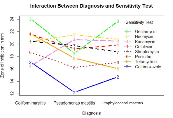
An interaction plot was generated to describe interaction between the two main factors; diagnosis and sensitivity.

interaction.plot(x.factor= Mastistis_clean$Diagnosis,
                 trace.factor=Mastistis_clean$Sensitivity_test,
                 response= Mastistis_clean$Yield,
                 type="b", 
                 main="Interaction Between Diagnosis and Sensitivity Test",
                 xlab="Diagnosis",
                 ylab = "Zone of Inhibition in mm",
                 col = c("red","blue", "green", "violet", "gold", "brown", "black", "orange"),
                 lwd=3,
                 trace.label = "Sensitivity Test")

Interpretation

Gentamycin had the highest effects of all the sensitivity tests. Cotrimoxazole had the lowest effect. This could be attributed to high resistance of the pathogens to this anti-microbial agent.

There was an interaction of anti-microbial agents at different zones of inhibition. Cotrimoxazole and Kanamycin interacted at zone 17. Penicillin interacted with Kanamycin at zone 18 and Tetracycline at zone 17. Tetracyline interacted with Penicillin at zone 18, Kanamycin at zone 19, Streptomycin at zone 20. Neomycin at zone 21 and Cefalexin at zone 21. Gentamycin interacted with Neomycin at 21, Cefalexin at 21, Kanamycin at 20.

Moving across the diagnosis the study found the following; Gentamycin had highest effect on Coliform mastitis and Staphylococcal mastitis. There was a drop in the trend in Pseudomonas Mastitis indicating some of resistance. There was a general negative trend moving from Coliform mastitis to Pseudomonas Mastitis and a positive trend moving towards Staphylococcal mastitis for the sensitivity tests; Gentamycin, Cotrimoxazole, Penicillin and Cefalexin Tetracycline and Streptomycin exhibited a negative trend moving across Coliform mastitis and Staphylococcal mastitis. Kanamycin and Neomycin had a positive trend moving from Coliform mastitis to Pseudomonas mastitis. The trend was however relatively stable moving from Pseudomonas Mastitis to Staphylococcal mastitis

Conclusion

The factorial experiments are useful in that they allow us to analyze the effects of different factors simultaneously. The doebioresearch package contains numerous functions on how to analyze design of experiments data in biological research. We can analyze more than one dependent variable against various factors. Interaction plots visualize the interaction between to main factors. However, some may not clearly visualize the interaction. This does not mean that there are no interactions in the data.

References

Montgomery, D. C. (2012). Design and analysis of experiments. New York: John Wiley. Gomes F, Henriques M. Control of bovine mastitis: old and recent therapeutic approaches. Curr Microbiol. 2016;72:377–82. doi: 10.1007/s00284-015-0958-8. PubMed https://pubmed.ncbi.nlm.nih.gov/26687332/ Agricultural Statistics. Factorial RBD Analysis in 1 line along with LSD test in R [YouTube Video] https://youtu.be/8D2AFA3Dt8U Penn State University online lecture notes. https://online.stat.psu.edu/stat503/lesson/6

← Previous Post Next Post →

Analyzing Factorial Experiments in R

Manipulating Factorial Data Using the DoeBioeresearch Package

Introduction to Factorial Experiments

What are Factorial Experiments?

Advantages of Factorial Experiments Over One Factor at a Time Experiments

Disadvantages

Factorial Designs Using R

Example 1

Loading the data and required packages

Some Visualizations

Running a factorial experiment.

Hypotheses

Result Interpretation

Are the concentration (Block) significant?

Are the Effects of the Extracts Significant?

Are the Effects of the Bacteria Significant?

Are the Two-Factor Interaction Effects Significant?

Treatments

Bacteria

Interaction Effects

Checking for interaction within the data

Example 2

Loading the Data and some required packages

Some Exploratory Data Analysis

Aggregation by Isolates

Dropping values with No isolates

Cummulative Yields for the Zone of Inhibitions

Analysis of Diagnosis and the Anti-microbial Agents

Hypotheses

Interpretation of the ANOVA Results

Main Effects

Interaction Effect

Interaction plot

Interpretation

Conclusion

References